Deciphering Ecuadorian Retail Trends: A Time Series Forecasting Approach to Sales Prediction

                                                           Photo by Isaac Smith on Unsplash

Beyond the bustling aisles and checkout lanes of grocery stores, there lies a complex web of purchasing patterns, seasonal trends, and intricate sales dynamics. Understanding and predicting these dynamics can be the key to a retailer's success or downfall. For Corporation Favorita, one of Ecuador's largest grocery retailers, these patterns translate to thousands of items across multiple store locations. With the rise of data science and advanced analytical techniques, time series forecasting has emerged as an invaluable tool for businesses like Favorita. It is used in the studying of past data and makes predictions about future time points. This model informs businesses when making stocking decisions, strategizing promotions, and optimizing the supply chains. In this article, we embark on a journey to harness the power of time series forecasting, aiming to craft a robust predictive model that can more accurately forecast the unit sales of Favorita's vast product range across its numerous stores. We would also be adopting the CRISP-DM framework approach for this project .

BUSINESS UNDERSTANDING

Predicting the future isn't the sole challenge. Understanding the 'why' behind sales trends is equally crucial. For companies like Favorita, this is where regression analysis steps in, bridging the gap between forecasting and understanding. Regression analysis stands out as a robust and powerful statistical technique, offering significant insights when evaluating retail sales dynamics. With its capacity to decipher the key influencers of sales, to accurately project future sales trends, and to guide decision-making in areas like store operations, merchandise choices, pricing strategies, and promotional campaigns, it is indeed a must-have tool when crafting detailed models that offer invaluable insights.

To harness the full potential of regression analysis in understanding retail sales, one needs to start by gathering pertinent data. The cornerstone of this process is distinguishing between the dependent variable, which is the sales, and the independent variables. These independent variables represent potential driving forces or influencers we feel might be affecting the sale sales outcomes.

Having sculpted a regression model with the data at hand, the gateway to valuable insights opens. Not only can you project sales for upcoming periods with heightened accuracy, but the model will also shine a light on the most influential factors shaping sales outcomes. This, in turn, becomes instrumental when strategizing on effective ways to elevate sales performance.

DATA UNDERSTANDING

Before embarking on our project, securing the right datasets was very necessary. We meticulously sourced our data from three key locations:

 

 - GitHub: A hub/cloud space for collaborative projects and version-controlled repositories. 

- OneDrive: A cloud storage solution ensuring seamless team access and collaboration. 

- Databases: Our primary reservoir for structured and direct data queries.

 

 The datasets acquired, pivotal to steering our analysis in the right direction, encompassed: 

 1. Store Dataset: A detailed insight into individual stores, shedding light on their specific locations and corresponding cities. 

2. Holiday and Events Dataset: This dataset chronicles the myriad holidays and events in Ecuador. Importantly, it discerns which holidays had broader implications on sales and operations. 

3. Train Dataset: The backbone of our analysis, this data serves as the training ground for our predictive models.

 4. Test Dataset: A comparative tool, it mirrors our training set, but with the exclusion of the all-important target variable. 

5. Oil Dataset: This dataset is a daily tracker of oil trends and prices, crucial given the fluctuating nature of oil markets. 

 To ensure we were primed for the analytical tasks ahead, an in-depth preliminary review of each dataset was undertaken. This allowed us to understand the scope and nuances of the data at our disposal. After our review, we observed that all the dataset were complete except the oil dataset which was incomplete(missing values). From the stores dataset, we realized that the brand Favorita was present in just 22 cities but in 16 states across the country and  Favorita boasts an impressive network of 458 stores.. Observing the holiday and event dataset, we again realized that of all the 350 holidays recorded over a period of 4-5 years, only 103 were unique and 72 of these were national holidays. We observe that sales really soar during the end of the year possibly due to the Navidad holiday and festivities and plummet again during the first week of the year. There's also a slight peak during the month of April, May , June. The sales for the rest of the years just oscillate between high and low. We can observe a yearly seasonality trend at play.

| Type of Holiday  | Unique Count | Total Count |

|------------------|--------------|-------------|

| Local Holidays   | 27           | 152         |

| National Holiday | 72           | 174         |

| Regional Holiday | 4            | 24          |

| **Total**        | **103**      | **350**     |

| Entity         | Count |

|----------------|-------|

| Cities         | 22    |

| States         | 16    |

| Shops          | 458   |

EXPLORATORY DATA  ANALYSIS

Following our meticulous review of the datasets, certain pressing questions naturally emerged. These queries were pivotal, shaping the trajectory of our subsequent analyses. By juxtaposing the sales column against other features, our objective was to discern which elements had the most profound influence on sales outcomes. This preliminary assessment led us to form an initial hypothesis. This educated conjecture would later serve as the foundation upon which we'd either validate our assumptions or debunk them during our deeper analytical dives. We encapsulated our hypothesis and key research questions as follows:

Hypothesis:

H0: Changes in the price of oil and the presence of holidays affects amount of sales made by stores.

H1: The price of oil and the presence of holidays does not affect the amount of sales made by stores.

Data Mining Goals & Research Questions

SALES TRENDS

1. How have sales trends evolved over the years? Are there seasonality patterns?

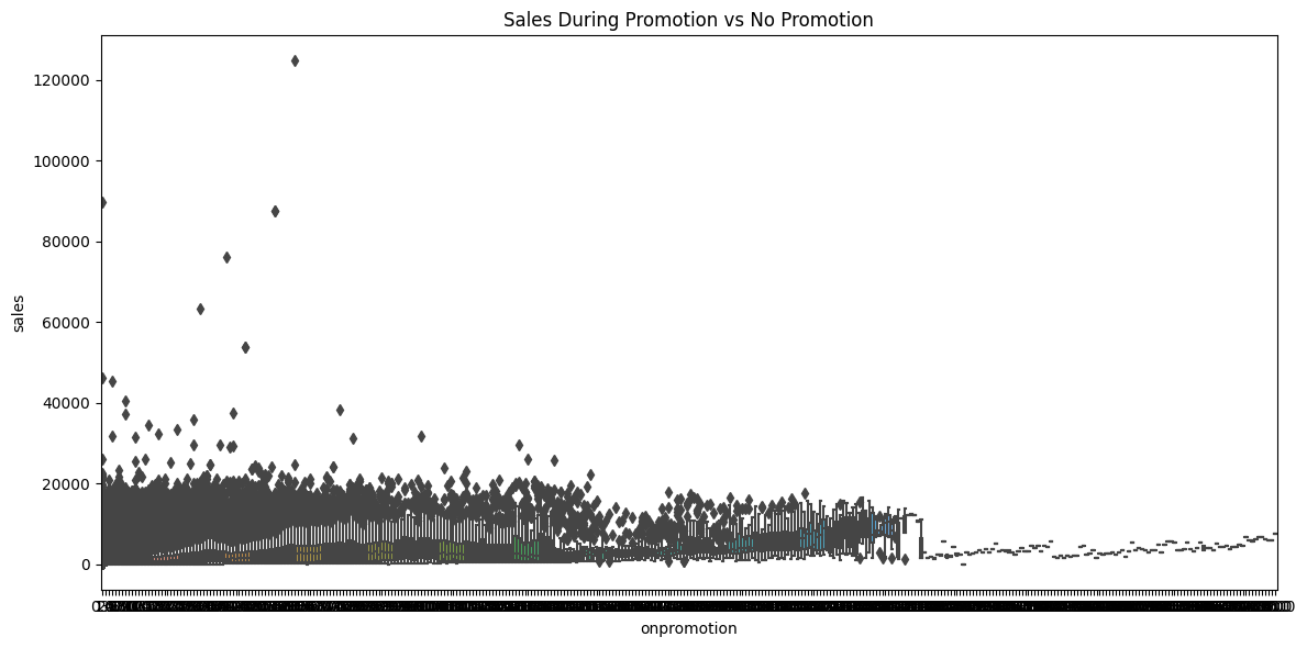
2. How do promotions impact sales? Is there a significant spike in sales when products are on promotion?

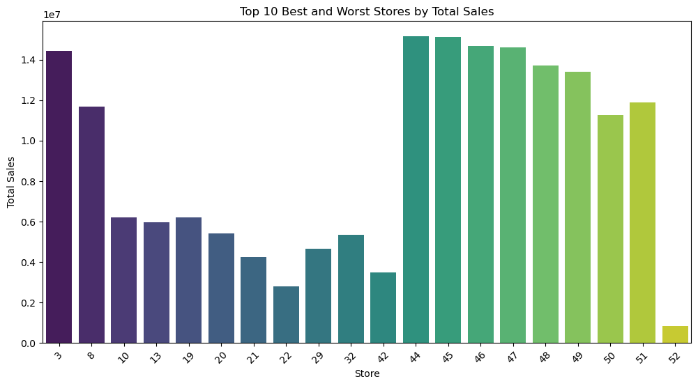
3. What are the top 10 best/worst stores and their best selling products?

4. How do transactions correlate with sales? Do more transactions always mean higher sales?

HOLIDAYS&EVENTS ANALYSIS

5. How many holidays/events occur on a local, regional, or national scale?

6. How did the earthquake on April 16 2016 impact sales?

OIL PRICE ANALYSIS

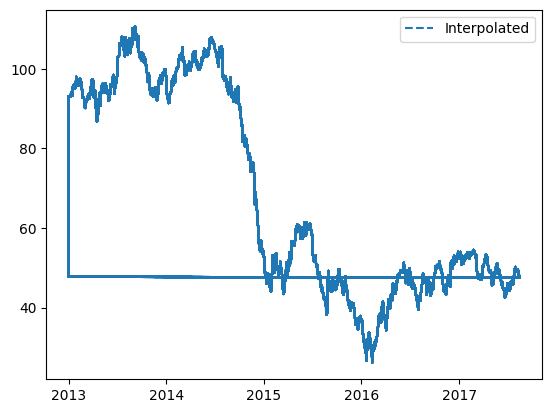
7. What is the trend in oil prices over time?

8. Are there specific months or periods when oil prices spike or dip?

Subsequent to these guiding questions, it was evident that predicting sales was not going to be a straightforward task as it seemed quite layered and multifaceted. Various external and internal factors, ranging from holidays to oil prices and product categories, weigh heavily on sales figures. Given that these influential attributes are scattered across different datasets, piecing together a comprehensive analysis becomes a demanding endeavor. This fragmentation necessitated the consolidation of these datasets into a single, cohesive unit for a streamlined analysis.

However, the challenge wasn’t just merging the datasets; the crux lay in determining the criteria or metrics for this consolidation.

To address this, we created a new dataframe titled 'nu_data'. Leveraging the common 'date' column, we merged the oil and holiday events datasets into 'nu_data' using an outer join. Recognizing that the train dataset would be central to our analyses, we established a consistent date range based on it. This preemptive step simplified the subsequent merging process. Following this, 'nu_data' was seamlessly combined with the 'stores' dataset to yield our final, comprehensive dataframe.

Given the vastness and complexity of the data, missing values were an expected challenge across multiple columns. To ensure data integrity and consistency:

- Flags and fill methods addressed most missing values across the columns.

- For the 'sales' column, forward fill was employed to substitute the missing values.

- For the 'oil' column (specifically 'dcoilwtico'), we integrated interpolation combined with backward fill to handle gaps in the data.

This meticulous data preparation and integration approach ensured that our final dataset was robust, comprehensive, and primed for in-depth analyses.

After our univariate analysis, during the exploratory data analysis phase, we moved to answering of the questions we asked during the beginning of the EDA phase, the resulting graph for each question is found below , also , the codes to each question can be found on this github repo https://github.com/florenceaffoh/LP3-TimeSeriesAnalysis/tree/master.

1.

A close examination of the graph provided an intriguing narrative of the company's sales journey over the years. The fluctuations in sales are both revealing and instructive:

• 2013's Stability and Surge: The year began on a stable note, with sales maintaining consistency for a good duration. However, as the year drew to a close, a significant surge was observed, carrying the momentum into the early parts of 2014.

• 2014's Rollercoaster Ride: This year was marked by volatility. While sales experienced several peaks and valleys, the most pronounced dip was observed towards the year's end. This downturn extended well into the initial parts of 2015.

• 2015's Recovery: After the considerable slump in the early months, sales began a steady recovery, regaining stability towards the latter part of the year.

• 2016's Mid-Year Challenge: The newfound stability continued into the first half of 2016. However, mid-year brought with it another dip. Fortunately, this was short-lived.

• 2017's Consistent Performance: This year marked a return to consistent sales, with the company maintaining a relatively even trajectory throughout.

The graph underscores the company's resilience, highlighting periods of challenge, recovery, and sustained growth.

2.

Upon examining the plotted data points, it's evident that there isn't a discernible linear trend between sales and promotional activities. The scattered distribution of points suggests a weak correlation between the two variables. Thus, it might be inferred that promotions might not have a strong direct impact on sales, at least not in a consistent and predictable manner.

3.

5.

4.

The scatter plot illustrates a general trend where sales tend to increase with a rise in transactions. However, it's crucial to note that there is substantial variability among the data points. This variability implies that while transactions indeed have an influence on sales, other factors are at play as well, contributing to the fluctuations in sales. In essence, transactions are a significant factor but not the sole determinant of sales, suggesting the presence of additional variables influencing the outcome.

6.

Post the 2016 earthquake, sales data revealed a significant uptick, hinting at the disaster's deep influence on consumer purchasing patterns. This surge can be attributed to immediate needs for essentials, transportation disruptions prompting bulk buying, the community's reconstruction phase, emotional buying responses, and the injection of insurance claims into the market. Understanding these shifts helps businesses adapt effectively to such unexpected challenges.

7.

8. 

FEATURE SELECTION AND MODELLING

As we transitioned into the subsequent phase of our analysis, we implemented a few critical steps to ensure data integrity and quality:

1. Backup Creation: First and foremost, we duplicated our existing dataframe. This proactive measure ensures that, in case of any inadvertent missteps or errors, we have a reliable backup to revert to, preserving the original data structure.

2. Feature Selection: With the goal of refining our model, we cherry-picked the most relevant features. All of these selected features were housed in a copied dataframe dubbed "nu_data1".

3. Date Manipulation: Recognising the importance of chronological data, we converted the 'date' column from its original object type to the more apt datetime format. Simultaneously, we elevated this column to an index, laying the groundwork for time series analyses.

4. Outlier Management:Outliers, while sometimes disruptive, can also carry valuable information. Instead of outright discarding them, we chose a more nuanced approach: winorization. This technique caps the outliers, thus preserving the data's structure and essence without letting extreme values skew our analyses.

5. Data Extraction and Resampling: We filtered our desired columns from "nu_data1", namely 'sales', 'onpromotion', 'hol_type', and 'transferred'. To align our data with daily rhythms, we resampled it at a daily frequency. For the columns 'sales' and 'onpromotion', we opted for aggregation through summation to capture the day's total activity.

6. Date Decomposition: Leveraging the richness of the date data, we decomposed it into three separate columns: day, month, and year. This allows for granular analyses based on different timeframes.

These structured preparations lay a solid foundation, ensuring our model is trained on clean, relevant, and insightful data.

To achieve a deeper grasp on the dataset's underlying patterns, several strategic adjustments and analyses were made:

1. Monthly Resampling: Initially, the resampled data's frequency was shifted to a monthly scale. This granulation aids in discerning broader trends and patterns that might be obscured at a daily level.

2. Seasonal Decomposition: Delving further into the temporal dynamics, a seasonal decomposition was performed. By breaking down the time series data into its constituent parts and plotting the seasonal decomposition components, we could unveil the inherent seasonality, trend, and residual components.

3. Autocorrelation Insights: To tap into the internal relationships within the time series data, both the Autocorrelation (ACF) and Partial Autocorrelation (PACF) graphs were plotted. These tools provide a window into the time-dependent structure of our series, illustrating the AutoRegressive (how the series correlates with its lagged values) and Moving Average (how the error term correlates with its lagged values) elements.

4. DataFrame Allocation: The resampled dataset was assigned to a new dataframe termed "df_resample." A notable feature of the resampling process is its automatic handling of missing dates, either imputing or interpolating values as needed to maintain continuity.

1. ACF Insights (Moving Average - q): The ACF chart helps in determining the Moving Average component of a time series. In our data, we note that all lags seem significant, as they lie above the significance level. However, the lags at positions 1, 6, 7, and 8 are especially pronounced. This suggests a potential MA(1), MA(6), MA(7), or MA(8) component in the data.

2. PACF Insights (Autoregressive - p): The PACF chart sheds light on the Autoregressive component of the series. In our analysis, the lags at 1, 4, 6, and 7 stand out as they notably exceed the significance level, hinting towards a potential AR(1), AR(4), AR(6), or AR(7) component in the data.

Given these observations from both ACF and PACF, a plethora of model combinations can be considered for forecasting. Models like ARIMA (Autoregressive Integrated Moving Average) can be tuned using various p and q values as gleaned from the PACF and ACF charts, respectively. Experimentation with different combinations can lead to the identification of the most fitting model for our data.

Moving Average (MA) plots serve as powerful tools in time series analysis, acting as smoothing agents that help mitigate short-term fluctuations and bringing underlying trends to the forefront.

By employing MA plots, we can effectively tame the 'noise' in our dataset, enabling a clearer view of its intrinsic movement. This process offers an enhanced understanding of data behavior, highlighting any consistent inclines, declines, or stable patterns.

For our current analysis, we will further refine this approach by plotting the moving average on an annual basis. By doing so, we can emphasize and distinctly visualize any long-term trends that emerge over each year.

In essence, MA plots, especially when broken down by year, offer a distilled and comprehensible view of our data's trajectory, facilitating informed future predictions and analyses.

1. Data Partitioning: We began by splitting our dataset into 'train' and 'test' segments. This separation facilitates both model training and subsequent validation.

2. Statistical Models for Univariate Data:

   - Using only the 'sales' column with the date as our index, we first delved into univariate time series forecasting.

   - Guided by insights from the ACF and PACF charts, we explored the AR model, ARIMA, and SARIMA:

     - For the ARIMA model, a systematic approach was employed to pinpoint optimal p, d, and q values. Our aim? To minimize the AIC. The AIC not only assesses model fit but also takes into account model complexity, making lower values desirable as they indicate a balanced model.

3. Regression Models:

   - We shifted gears to delve into machine learning, exploring models like XGBoost, K-Nearest Neighbour, Random Forest, and Linear Regression.

   - After encoding relevant columns, we partitioned our data, setting aside 'sales' as our target variable, y.

   - Models were trained and subsequently evaluated using metrics such as MAE, MSE, RMSE, RSE, and RMSLE. These metrics shed light on model accuracy and reliability.

   - Post-training, the models were deployed on the test set, furnishing forecasted values derived from learned patterns.

4. Model Evaluation and Refinement:

   - If initial results weren't satisfactory, we were poised to recalibrate. Options on the table included parameter adjustments, model substitutions, or even re-examining data preprocessing.

   - Upon analysis, the standout performers were the XGBoost and Random Forest Regressor models, with RMSLEs of 0.2359 and 0.2371, respectively.

5. Hyperparameter Tuning:

   - Recognizing the potential of our top performers, we dove into hyperparameter tuning. This fine-tuning process aims to squeeze out the best performance by optimizing model settings.

This rigorous process, replete with iterative refinements, ensured that we not only had models that captured data nuances but also were primed for accurate future predictions.

RECOMMENDATIONS AND CONCLUSION

Working on this project has so far been a bit challenging as it wa quite a diversion from what we were used to but also one of our best and most interesting work so far as we got to learn a lot about the brand Favorita and the country Ecuador . So based on our analysis and what we have learnt so far, if a similar brand wants to learn from these analysis or Favorita wanted to implement some changes, these are what I would recommend:

Response to Natural Disasters and Unforeseen Events:

1. Inventory Management: Anticipate a surge in essential goods demand during crises to avoid supply chain disruptions and meet consumer needs.

1. 1. 2. Psychological Impact: Recognize post-disaster behavioral changes and cater to potential increased demands, as some might resort to shopping as a coping mechanism. 3. Insurance Payouts:Understand that post-disaster insurance compensations can lead to increased purchasing power, influencing sales dynamics. 4. Community Engagement:Participate in CSR initiatives post-disasters, benefiting the community and bolstering the company's reputation. Insights from Sales Patterns: 5. Detailed Analysis of Dips: Investigate the reasons behind significant sales decreases to strategize against similar future challenges. 6. Seasonal Trends: Recognize and capitalize on seasonal sales surges, like the end-of-year boosts, for efficient planning. 7. Customer Feedback and Market Research:** Regularly gauge customer preferences and sentiments to understand sales trends, especially during volatile periods. 8. Operational Audit:Regularly review operations, contrasting performances during stable times and dips, to highlight areas of improvement. Proactive Business Strategies: 9. Diversify Offerings: Based on consistent sales data, expand or diversify product lines and revamp underperforming offerings. 10. Risk Management: Develop a strategy to anticipate and mitigate potential risks affecting sales. 11. Strengthen Supply Chain:Build a resilient and adaptive supply chain to navigate external challenges effectively. 12. Regular Forecasting:Use advanced tools for more accurate sales forecasting, aiding better decision-making. 13. Promotional Strategies: Implement promotional campaigns or loyalty programs during sales dips to boost recovery. 14. Stakeholder Communication: Ensure transparent communication with all stakeholders to keep them aligned with the company's vision and strategies. By adopting these strategies, businesses can not only navigate challenges but also position themselves for sustained growth.

      
      

      You can find the code to the project on my GitHub repo https://github.com/florenceaffoh/LP3-TimeSeriesAnalysis

      
      

      thank you